ZScope

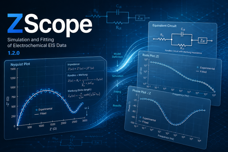
Publication-Grade Electrochemical Impedance Spectroscopy Platform

         

Story · What's New · Capabilities · Workflow · Benchmarks · Applications · Comparison · Installation · Citation

---

🔬 The Story Behind ZScope

ZScope was not designed in the abstract. It was born from a real experimental problem.

During an electrochemical study, I needed to capture a baseline EIS spectrum at the start of a reaction — then measure six more spectra at different oxidation states as the reaction progressed. Each spectrum represented a distinct state of the system, and together they told the story of a mechanism evolving in time.

The analysis became a frustration. Working through seven spectra with existing tools was slow, disjointed, and offered no intuitive sense of how parameters evolved across the series. There was no way to interactively explore the relationship between circuit components and spectrum shape — to build the physical intuition that makes EIS meaningful.

I kept thinking: what if I could draw a circuit, move a slider, and watch the simulated Nyquist plot respond in real time — overlaid on my experimental data? Not as a fitter, but as a lens for understanding. A way to arrive at a physically motivated starting point before handing off to a numerical optimizer.

That idea became the first version of ZScope.

As the tool took shape, it grew. The fitting engine followed — built with the same insistence on reliability and physical transparency. Then Bayesian uncertainty quantification, because a parameter without an honest uncertainty estimate has limited scientific value. Then data validation, custom components, automatic circuit suggestion, and structured reporting.

ZScope is the tool I needed during that experiment. It is free, and I hope it gives other researchers something better than what was available to me.

Distribution: ZScope is released as a ready-to-install application for Windows. Source code is not publicly distributed. Full scientific documentation, validation benchmarks, and an in-app help manual are provided so you can trust what happens inside.

---

🚀 What's New in 2.2.0

Save & Open Project — an entire session now lives in one .zscope file: every loaded dataset with its circuit, its fit and Bayesian results, its DRT analysis, and its import column mapping. Reopen it and everything is where you left it. The file is an ordinary ZIP archive with a readable JSON manifest inside, so it can be inspected without ZScope, and numerical arrays are stored exactly — a reloaded project is bit-for-bit identical to the one you saved.

Export datasets as separate project files — split a batch into one independently-reopenable project per dataset. Unlike CSV export, each file keeps that dataset's circuit, fit and DRT results with it.

Paste data from the clipboard — copy a block of cells in Excel, LibreOffice, Origin or a text editor and press Ctrl+V; the import dialog opens on the pasted table. Separator and decimal convention are detected automatically, including semicolon-separated European exports with decimal commas (1,0E+05;10,5), which a naive parser reads off by a factor of ten. Pasted data is written to a timestamped file so it can be re-examined and embedded in a project, rather than living only in a clipboard buffer.

Import many files at once — select or drag in a whole folder of spectra. ZScope reads each one, detects its columns, and shows a review list with point counts and frequency ranges before anything loads. Files from the same instrument share a layout, so a typical batch needs one click; anything that needs attention opens the full import editor on its own, and one file's mapping can be applied across the whole batch.

Import source tracking — every spectrum records how it was obtained: columns detected automatically, columns chosen by you, or data values edited by hand. It is shown during import, written to the log, and saved into the project file — so months later it is still answerable which curves are the file as measured, and which carry a human decision.

Drag and drop now asks — dropping files offers Add (keep what is loaded and compare) or Replace (start over). Closing the application offers to save unsaved work first, and the window title marks a session that has any.

Note: DRT results were previously held only for the active dataset and were silently discarded when you switched datasets. They now belong to their dataset, follow it, and save with the project.

Previously — What's New in 2.1.0

AI-enhanced circuit proposer — local and online AI now assist the proposer in analysing your spectrum and suggesting equivalent circuit models. The underlying proposer architecture was also reworked for better baseline accuracy independently of AI.

Bring your own AI account — import and connect a personal or enterprise AI account to power the proposer.

New benchmark suite — integrated benchmarks for rigorously evaluating, comparing, and validating circuit model performance.

Upgraded Fitting, DRT and Kramers–Kronig evaluation — improved accuracy, better edge-case handling, and more robust metrics across all three.

Major fitting speed-up for large circuits — the Trust-Region Reflective bottleneck is resolved. The Jacobian is now derived analytically from the circuit rather than approximated by finite differences, costing one linear solve instead of one per parameter. Circuits with 10+ free parameters fit roughly 20–35× faster, with equal or better final fit quality.

Note on uncertainties: two corrected defects affected reported ± intervals on multi-arc circuits and on circuits containing an inductance. Fitted parameter values are unchanged. If you have drafted uncertainties from such fits, please re-run them.

---

⚡ Key Capabilities

🖥️ Real-Time Interactive Simulation The feature that started it all. Draw an equivalent circuit on the visual canvas, set your parameters, and the Nyquist, Bode, and Phase plots update instantly — with your experimental data overlaid. Adjusting Rct, CPE exponent, or Warburg coefficient by hand and watching the spectrum respond builds the kind of physical intuition no black-box fitter can provide. Drag-and-drop canvas with grid snapping Presets: Randles, Randles+Warburg, CPE variants, inductive loops, battery (FLW), Gerischer Save your own circuits to a personal library Circuit notation input/output (Rs-[Rct/Cdl]-W)	📥 Flexible Data Import Import EIS data without fighting file formats. ZScope recognizes the native export formats of most common potentiostats — Gamry, BioLogic, Autolab, Zahner, Ivium, CHI, PalmSens, PAR, and more — and falls back to a smart generic parser for anything else. Batch import: many files at once, columns auto-detected per file Paste tabular data straight from a spreadsheet (Ctrl+V), locale-aware Auto-detection and consistency cross-check of column pairs Sign convention toggle for different potentiostats Row-level filtering: exclude drift, artefacts, or outliers while keeping them visible Frequency sub-band restriction for fitting
✅ Kramers–Kronig Validation Before fitting any parameters, confirm your data is worth fitting. ZScope reconstructs Z(ω) from a Voigt (RC-ladder) basis that is KK-consistent by construction, with modulus weighting, a padded time-constant grid, and a series-inductance term to absorb ordinary cable inductance. You get a banded verdict from the median relative residual, plus a residual-vs-frequency diagnostic plot — a systematic trend in the residuals points to drift or non-stationarity, while random scatter is just noise. Residual Status Action < 0.5% ✅ Valid Proceed 0.5–2% ⚠️ Minor drift Narrow frequency range > 2% ❌ Violation Repeat measurement One keystroke (Ctrl+K), under 2 seconds.	🎯 Advanced Fitting Engine An escalating optimizer: exact, inexpensive methods first — global search engaged only when a fit fails quality acceptance, never as a routine tax on every run. Analytic Jacobian — the circuit's derivative in closed form via adjoint sensitivity, not finite differences LHS multi-start — Latin Hypercube Sampling, candidates screened before full refinement TRF — Trust-Region Reflective for gradient-precise local convergence DE escalation — Differential Evolution plus global restarts, triggered only on a rejected fit $$\chi^2 = \sum_{k} \frac{(Z'_k - \hat{Z}'_k)^2 + (Z''_k - \hat{Z}''_k)^2}{|Z_k|^2}$$ Modulus weighting · Soft-L1 robust loss · AIC/BIC model selection · Warm-start for series measurements (60–80% speed gain)
📊 Bayesian MCMC Uncertainty A single point estimate is not enough. ZScope uses the emcee affine-invariant ensemble sampler to map the full posterior distribution P(θ | Zexp): 95% credible intervals — probability-direct, not frequentist approximations Measurement noise scale is marginalised analytically rather than plugged in as a point estimate, so intervals account for uncertainty in the noise level itself The model's own posterior estimate of the noise level is reported — an independent check on calibration Marginal and joint posterior distributions Parameter correlation and covariance analysis Convergence diagnostics: R̂ (Gelman–Rubin) + autocorrelation time Predictive uncertainty bands from 300 posterior draws	🔧 Extensible Element Library Element Physical Meaning R, C, L Resistance, capacitance, inductance CPE Surface roughness / inhomogeneity W (Warburg) Semi-infinite diffusion FLW / FSW Finite diffusion (permeable/blocking) Gerischer Diffusion + chemical reaction Transmission line Porous electrode models Custom Any Z(ω) or Y(ω) expression Custom elements are defined through a GUI designer, exported as .json, and behave identically to built-ins in all fitting and simulation contexts — no coding required.
💾 Projects & Session Persistence An analysis session is rarely finished in one sitting. Save Project writes everything — datasets, circuits, fits, posteriors, DRT results, import settings — into a single .zscope file that reopens exactly as you left it. One file per session, or one file per dataset Open ZIP container with a readable JSON manifest Arrays stored exactly: reload is bit-for-bit identical No pickled objects — a project file cannot execute code Versioned schema: projects stay readable as ZScope evolves	🔎 Data Traceability Every spectrum carries a record of how it entered the analysis — auto-detected columns, a mapping you chose, or values you edited by hand — visible during import, written to the log, and preserved inside the project file. Combined with embedded copies of the original source files, a .zscope project is a self-contained record of an analysis: the raw data, what was done to it, and the result.

---

🗺️ Recommended Workflow

  Load Data  ──▶  KK Validate  ──▶  Build Circuit  ──▶  Fit  ──▶  MCMC  ──▶  Export
      │                │                  │               │          │           │
  auto-detect      < 2 seconds       real-time sim    LHS+TRF+DE  posterior  txt/csv/
  column format    residual map      overlay data     warm-start   credible   json/PDF

1. Import — ZScope detects column format, cross-validates consistency, and lets you filter rows before any calculation. Import one file or a whole batch.
2. Validate (Ctrl+K) — Confirm linearity and stationarity; investigate flagged frequency regions
3. Build your circuit — Draw on canvas, choose a preset, or request an algorithmic suggestion based on spectral fingerprinting
4. Fit — Configure weighting, loss function, restarts, and frequency band; run the optimizer
5. Quantify uncertainty — Run Bayesian MCMC for full posteriors, credible intervals, and convergence diagnostics
6. Export — Publication-ready figures (PNG/SVG/PDF), parameter tables, structured reports — and a .zscope project preserving the whole session

---

📈 Validation & Benchmarks

ZScope is validated against synthetic data with known ground-truth parameters, across five reference circuits, three noise models, and multiple noise levels — over 19,000 independent fits per full benchmark run. Every figure below is a repeated-trial result with an interval, not a single-seed example.

Goodness of fit

χ² computed against the true per-point noise σ used to generate the data. A correctly-specified model fitted to the noise floor gives 1.0.

Noise level	χ²calibrated
2%	0.992
5%	1.006

Parameter recovery — blind start, 2% noise

Optimizer started from an uninformed guess (0.2×–5× per parameter), not from the true values.

Circuit	Worst parameter	Mean error
Randles	Cdl	0.36%
Randles + Warburg	σW	0.54%
CPE Randles	Q	1.79%
Two-Time-Constants	C₂	3.98%

All other parameters recover below 1%. The CPE exponent α recovers to 0.25%.

Confidence-interval coverage

Whether the reported ± actually contains the true value at its nominal rate — measured, not assumed.

Condition	Covariance estimator	Coverage (nominal 95%)
Well-behaved noise	Jacobian	94.4%
Well-behaved noise	Robust sandwich	93.1%
5% contaminated points	Jacobian	89.0%
5% contaminated points	Robust sandwich	94.2%

The robust loss is the shipped default: it costs about a point of efficiency on clean data and recovers calibration entirely when data contains outliers.

DRT resolution limit

How far apart two relaxation processes must be before the DRT resolves them as two peaks rather than one — the Rayleigh criterion analogue for impedance.

Noise	Required τ₂/τ₁
0%	≈ 10
1%	≈ 16
2%	≈ 27
5%	≈ 75

Approximately τ₂/τ₁ ≈ 15 × (noise level in %). Below the limit the method fails conservatively — returning a single peak at the geometric mean with the combined resistance, rather than inventing structure.

Where ZScope's methods have limits, the benchmarks report them. Kramers–Kronig testing reliably detects drift only once the distortion is large relative to measurement noise — a small drift is genuinely indistinguishable from noise, in any implementation. The Q–α correlation in CPE fitting reflects a real physical interdependence, not a software deficiency, and is detected and reported rather than hidden.

All benchmark data, comparison tables, and analysis scripts are available in benchmarks/ for independent verification.

---

🔭 Scientific Applications

Domain	Typical Use
Battery Science	SEI/CEI characterization · charge-transfer kinetics · Li-ion diffusion · state-of-health monitoring
Photovoltaics	Recombination dynamics · ion migration · hysteresis · capacitance spectroscopy
Corrosion Science	Polarization resistance · coating integrity · inhibitor screening · lifetime prediction
Fuel Cells & Electrolyzers	Ohmic · kinetic · mass-transport deconvolution in PEM, AEM, and solid-oxide systems
Supercapacitors	Double-layer behaviour · faradaic contributions · porous electrode transmission-line analysis
Bioelectrochemistry	Redox probe kinetics · biosensor interfacial impedance · biomolecular binding
Mechanistic Studies	Multi-state or time-series EIS — the exact scenario ZScope was designed for

---

🆚 Why ZScope?

Capability	Commercial Tools	Academic Scripts	ZScope
Real-time interactive simulation	Rarely	✗	✅ Instantaneous
Bayesian MCMC posteriors	Rarely	Manual	✅ Full emcee engine
Kramers–Kronig validation	Limited	Manual	✅ Integrated + residual maps
Global optimization (LHS+TRF+DE)	✗ Local only	Variable	✅ Escalating hybrid
Algorithmic circuit suggestion	Uncommon	✗	✅ Spectral fingerprinting
Custom elements (no coding)	Restricted	Script-level	✅ GUI designer
Sequential warm-start fitting	Rarely	Manual	✅ Automatic
Batch import of many spectra	Partial	Manual	✅ Auto-detected per file
Paste data from clipboard	✗	✗	✅ Locale-aware
Single-file session projects	Rarely	✗	✅ Open, inspectable format
Published coverage & resolution limits	✗	✗	✅ Measured and documented
Structured export (txt/csv/json/PDF)	Partial	Manual	✅ Full
Cost	💰 Annual license	Free	✅ Free

---

💾 Installation

Windows — Standalone Installer

⬇ Download Latest Release

No Python. No package manager. No dependencies. Download, run the installer, open ZScope.

macOS and Linux support are planned. If you work on those platforms, please open an issue — user demand shapes the roadmap.

---

📖 Citation

If ZScope contributes to published research, please cite it so others can find it:

@software{zscope2026,
  author  = {Mohammadi, Tecush},
  title   = {ZScope: Publication-Grade Electrochemical Impedance Spectroscopy Analysis Platform},
  year    = {2026},
  version = {2.2.0},
  url     = {https://github.com/Tecush/ZScope},
  doi     = {10.5281/zenodo.20357547}
}

DOI: 10.5281/zenodo.20357547

---

📬 Contact

Developer: Tecush Mohammadi Email: tecush@gmail.com GitHub: @Tecush Issues & feature requests: GitHub Issues

Questions about scientific methods, specific use cases, or validation data are welcome by email.

---

Built from a real experiment, for real researchers. Because good science deserves better tools.